Weather Regimes: The Atmosphere's Preferred Moods
Bio: Simon Lee is currently a Postdoctoral Research Scientist in the Department of Applied Physics and Applied Mathematics at Columbia University, working on large-scale extratropical weather and climate variability and predictability. He’s moving to the University of St Andrews (Scotland) in July, as a Lecturer (Assistant Professor) in Atmospheric Science.
During the course of a day, your mood might change several times – from the simple joy instilled by a great cup of coffee, to a transient flash of road rage. But over the course of several days to a week, one overall mood might characterise how you feel – perhaps you’re particularly satisfied with your job, or maybe you’re on vacation and feeling relaxed. Well, it turns out, the atmospheric flow also has such slowly-varying “moods”. These atmospheric moods are called weather regimes.
The idea behind weather regimes is that we can classify the atmospheric flow larger than individual weather systems into clusters, called regimes. You can think of it a bit like collections of moods that fall under the same umbrella. These regimes are recurrent (they happen repeatedly), persistent (they last for multiple days), and quasi-stationary (the pattern stays in the same place).
Classifying the atmosphere’s moods
By the mid-20th century, meteorologists in the UK had noted that certain types of weather seemed to persist longer than the individual weather systems themselves. These weather types were classified subjectively by manually inspecting weather charts (hard to fathom nowadays!).
As the 20th century progressed, a lot of work went into teleconnections – the idea that atmospheric circulation anomalies at one location are correlated with those far away. Some of these include the North Atlantic Oscillation (NAO) [no, not the Scottish band] and the Pacific-North American pattern.
Although teleconnections and regimes aren’t entirely unique concepts, teleconnections can only tell you about one part of the atmospheric flow at once. If you asked the atmosphere, “how are you feeling today?”, it could respond by telling you, “well, I’m feeling strongly PNA+ but slightly NAO-…” (and a whole host of other indices… let’s not worry about them). You would then have to work out what that combination meant for you (is the atmosphere actually in a good mood?). Alternatively, the atmosphere could have simply told you what the regime is: “I’m feeling Pacific Trough-y today”.
Looking under the hood, defining regimes usually involves some sort of clustering algorithm. The most commonly used is called k-means clustering. To use it, you give the algorithm the data you’re interested in organising, and tell the algorithm how many clusters (moods) you’d like. It then solves for the “centroids” (the centres of each cluster). In essence, each data point is assigned to a cluster, and the (squared) distance from the centre of that cluster is computed. By repeatedly trying different centroids, the algorithm eventually finds the centroids that minimise the sum of these (squared) distances. When finding weather regimes, 500 hPa geopotential height anomalies (i.e., mid-level pressure patterns) are usually used, since this field represents the large-scale variability in the troposphere well (and generally doesn’t run into any mountains).
Convergence of k-means clustering into three clusters. (Source: Wikimedia Commons)
Returning to the mood analogy, you can imagine this clustering procedure as being like grouping together all your specific moods into overarching mood states – for example, one cluster could contain all ‘sad’ moods, incorporating more specific feelings such as anxious, lonely, or frustrated (representing individual weather systems).
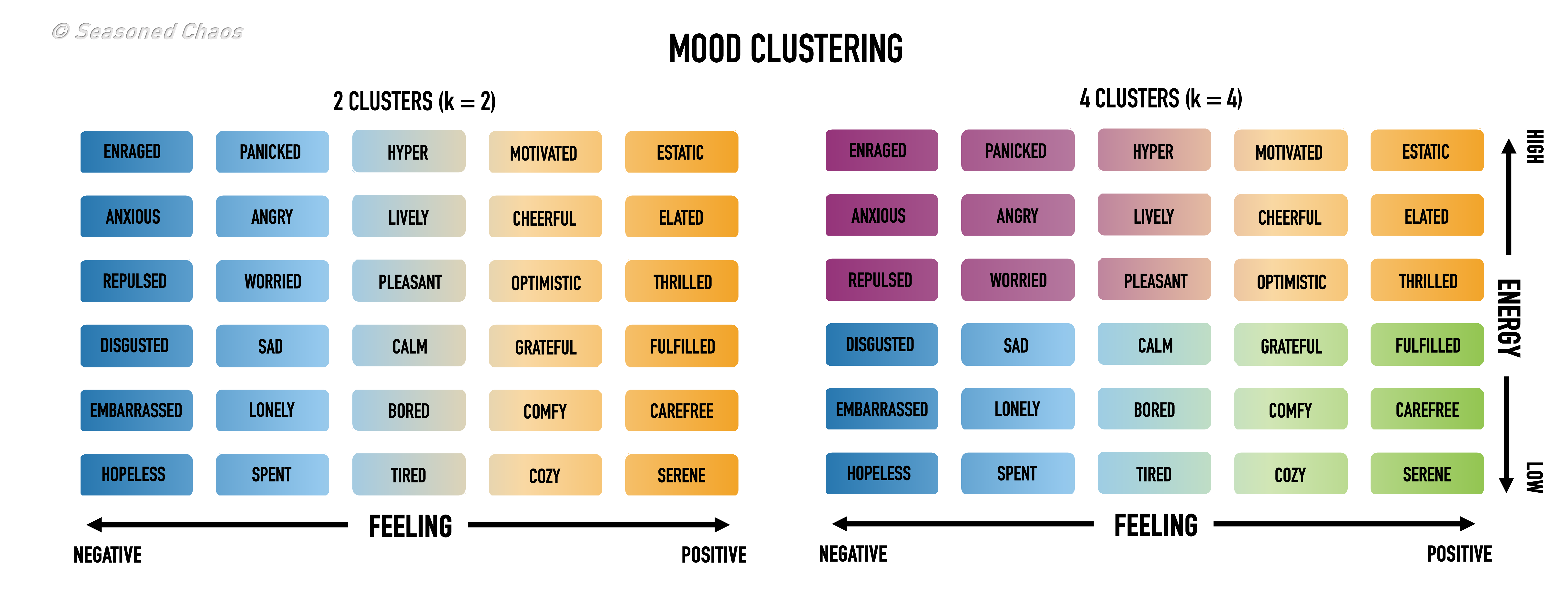
An example of how we can cluster moods into (left) two or (right) four mood ‘regimes’ – indicated by color shade – based on where the mood lies on philosophical axes of feeling (negative to positive) and energy (low to high).
The New Mood (year-round!)
Mid-latitude dynamicists have historically tended to focus on winter, because the variability is a bit more ✨ dramatic ✨, and phenomena like ENSO and the polar vortex are active and kicking the atmosphere into certain patterns. There’s already been a lot of work on wintertime weather regimes dating back to the 1980s. But, thankfully, winter is just one season! So how do we define regimes year-round? In a recent paper, we do just that and classify year-round regimes over North America. Let’s dig into some of the maths-y details…
Before attempting year-round regimes, we need to deal with the fact that there’s more atmospheric variability in the winter than the summer. This is important because we’re using a clustering algorithm that deals with variance, which would otherwise overemphasise winter and de-emphasise summer. Not good!
To get around that, we normalise the anomalies: we divide by the North America-average grid-point standard deviation of the anomalies for each day of the year. That’s quite a wordy sentence, but in simple terms this procedure means that k-means can treat winter and summer equally.
Now that we’ve dealt with the variability problem, the big question is: how many regimes? In our study, we performed various different tests and found that four regimes clearly emerged as the best solution. So, the atmosphere over North America has four ‘moods’! But what about those cases when the atmosphere isn’t in any particular mood – when the atmospheric flow isn’t anomalous? We reclassify these days as “No Regime”, and so we actually have five states:
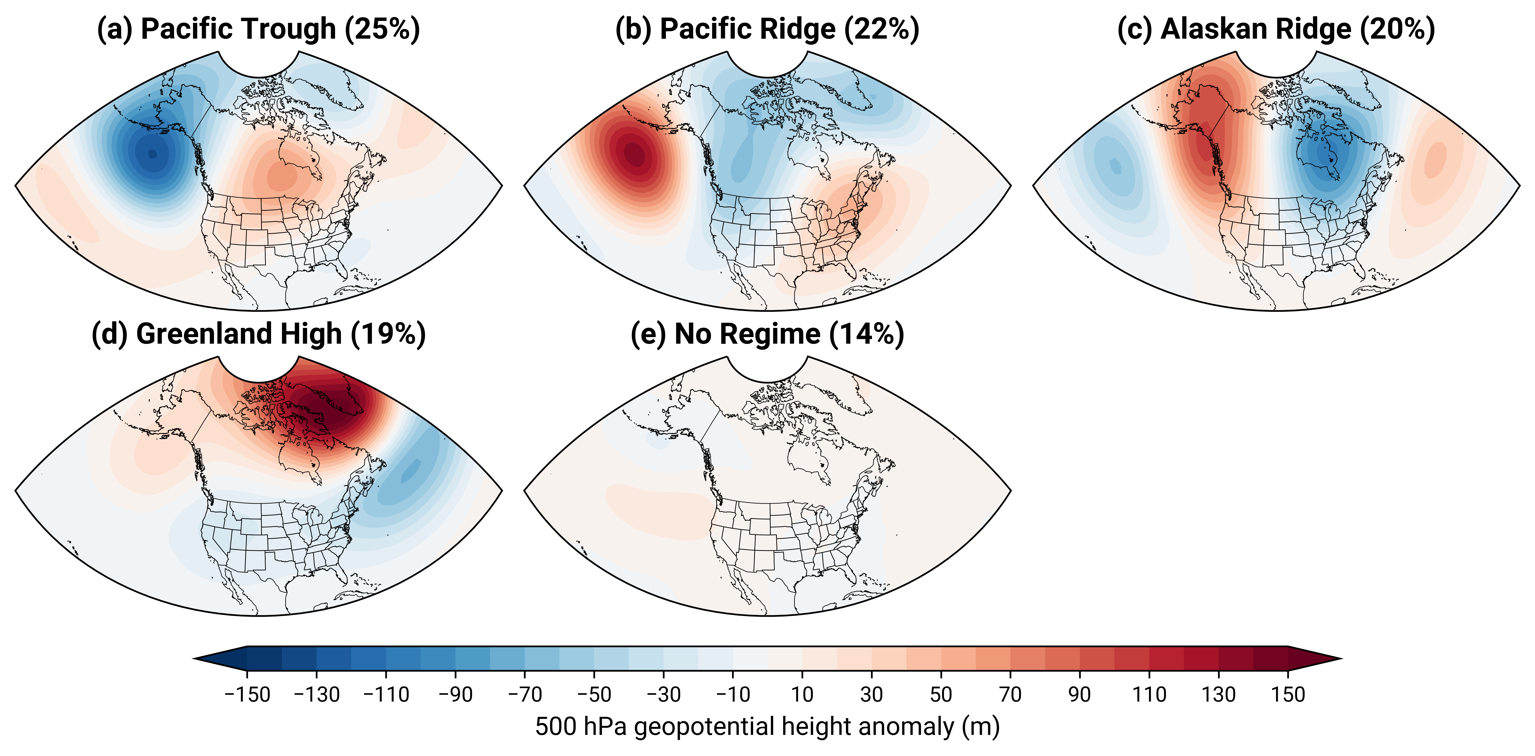
Average 500 hPa geopotential height anomalies during (a–d) four year-round North American weather regimes and (e) No Regime. The percent of days assigned to each regime are shown in brackets.
The Pacific Trough regime is known for supplying the West Coast with drenching atmospheric rivers, and is more common during El Niño. The Pacific Ridge regime is a bit of a chaotic player and often brings big temperature contrasts across North America – it is the coldest regime in the west and the warmest in the east – and is more common during La Niña. Alaskan Ridge likes to grab the headlines with cold air outbreaks, which it often brings to the eastern US and Canada, and drought in California. Meanwhile, Greenland High – which is similar to the negative NAO – is the one that East Coast snow lovers lust after, and is more common when the polar vortex is weak.
So what’s the point?
Interest in regimes has burgeoned alongside interest in subseasonal-to-seasonal (S2S) prediction. Regimes naturally sit somewhere between weather and climate, and so they can serve as one tool to ‘bridge the gap’ between the two. Previous studies have utilised regimes in understanding windows of opportunity for extended-range prediction and in diagnosing ‘flow-dependent predictability’, where forecast skill depends on the state of the atmosphere.
More generally, regimes serve as a simple and objective method for quickly interpreting the “big picture” from increasingly large ensembles, such as the 101-member, daily, 46-day forecasts from ECMWF. Using regimes means it only takes a forecaster a few minutes to gauge the mood of the atmosphere (present and future) in such large amounts of data. Take this example below, from the GEFS: Alaskan Ridge transitions into No Regime within the first week of the forecast, before a likely transition into Pacific Ridge by the end of February. Things then look more uncertain going into March, but the probability of Greenland High is above-normal while all other regimes are below-normal.
Is this a window of opportunity? Now that puts me in a good mood.
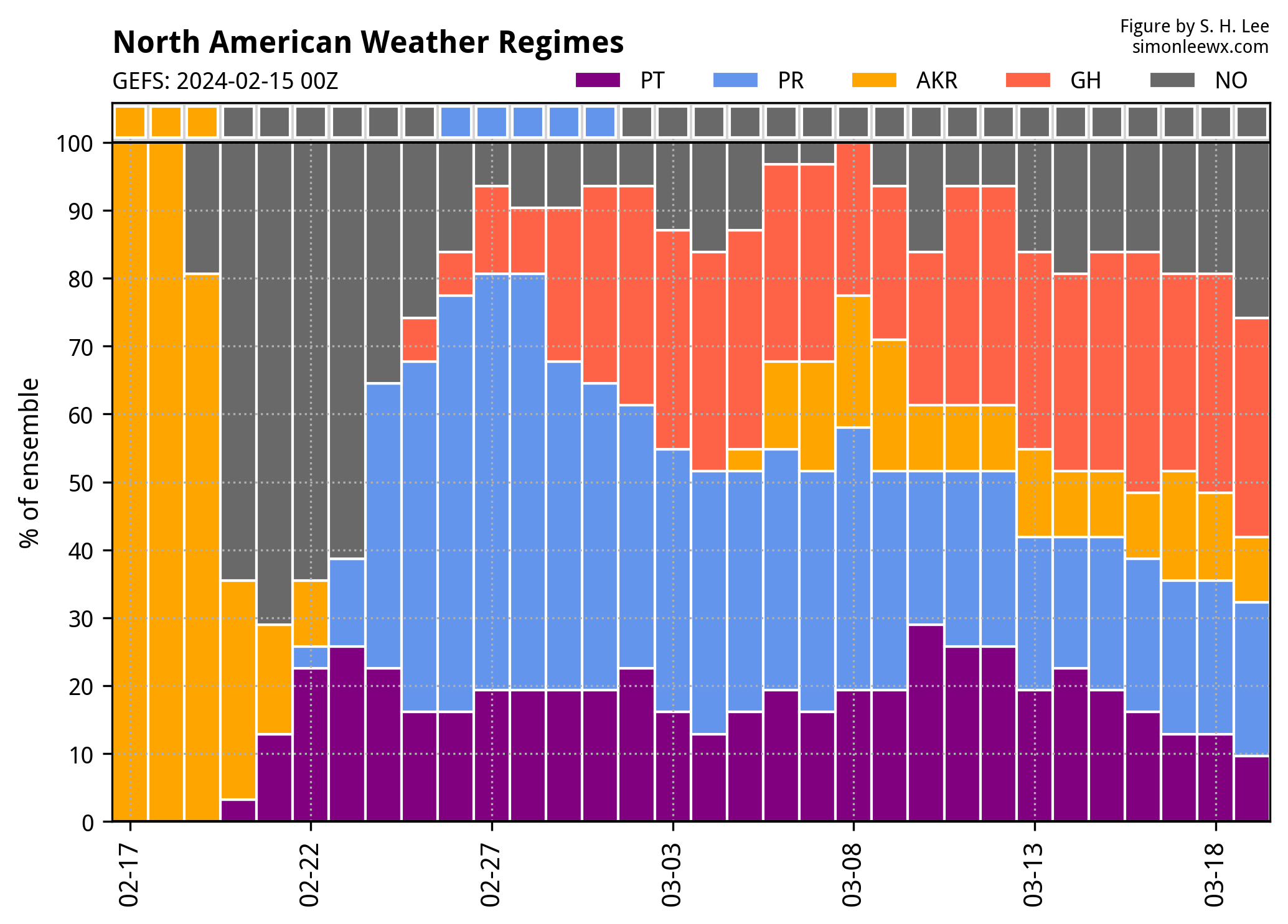
Global Ensemble Forecast System (GEFS) North American weather regimes, initialised on 15 February 2023. https://simonleewx.com/gefs_north_america_regimes/